phasefinder
phase prediction per best epoch
phasefinder is a beat estimation model that predicts metric position as rotational phase, heavily inspired by this paper.
Demos
`are you looking up`
mk.gee
`just the way it is`
action bronson
`lethal weapon`
mike & tony seltzer
`michelle`
the beatles
Why Phase?
Many beat estimation methods use binary classification (0,1) to detect ‘beat presence probability’.
This leaves the model without much context on the cyclical structure of music, i.e. it’s learning to flip a lever up & down at precise times.
In contrast, by estimating phase (the angle 0-360 where 0=beat, 360=next beat), every frame has meaningful information, e.g.
| binary | 0 | 0 | 0 | 1 | 0 | 0 | ... |
| phase | 312 | 328 | 344 | 0 | 16 | 32 | ... |
Instead of tracking onsets or learning the exact number of 0s between each 1, it only needs to look back a few frames to get an idea of the location and speed of the phase.
Rather than making discrete choices, it only needs to trace a continuous spiral through time.
Architecture
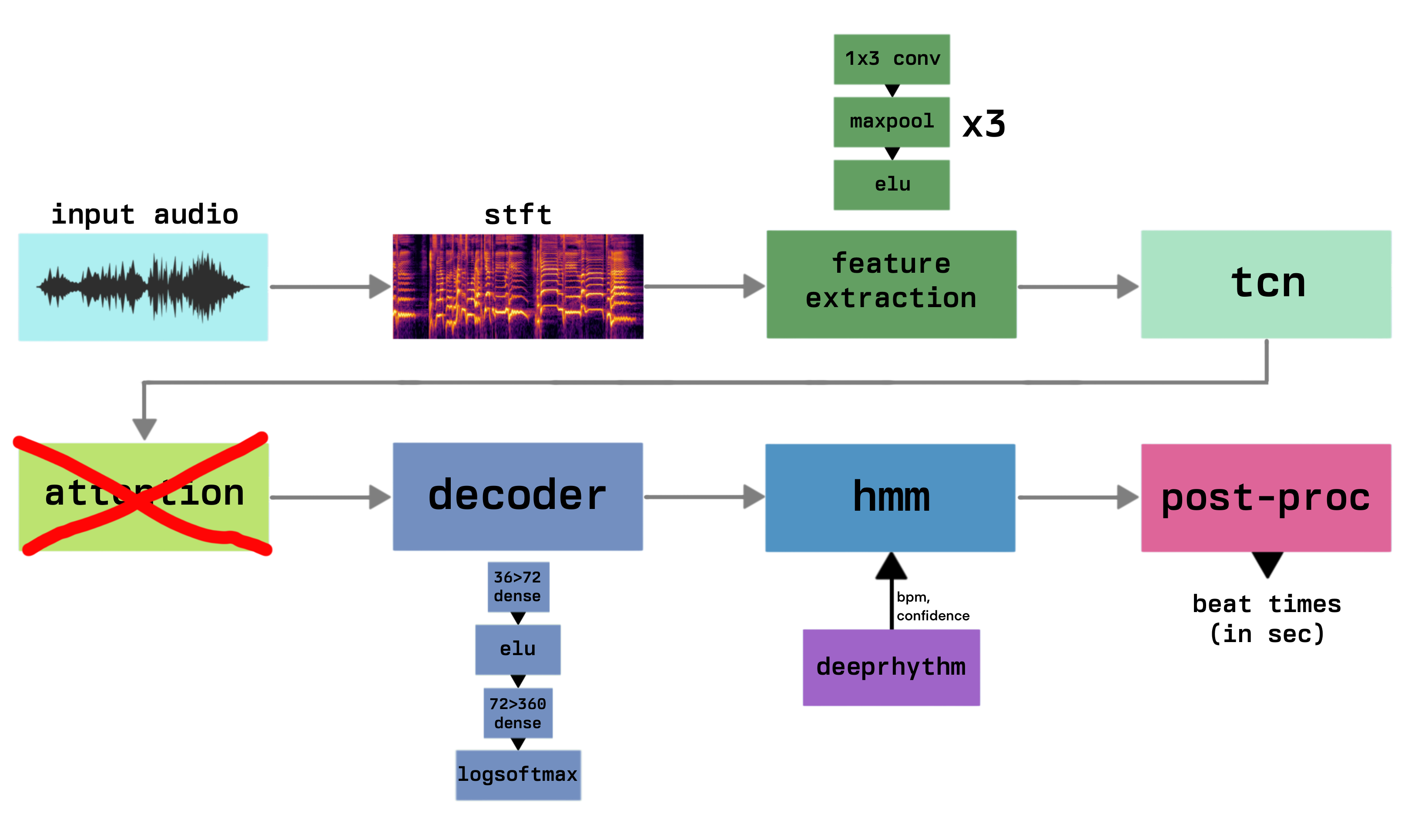
Input
- Audio, sampled at 22.1kHz
- Spectrogram with n_fft=2048 and hop=512
- Apply log filter, reducing frequency dimension from the original 1025 to 81 log-spaced bands
Feature Extraction
- Three 1D convolutional layers, each followed by max pooling, ELU activation, and dropout
- Starts with
num_bands(81) input channels and maintainsnum_channels(36) throughout - This setup reduces the frequency dimension while preserving temporal information
TCN
- Temporal Convolutional Network
- Consists of
num_tcn_layers(16) dilated causal convolutions - Uses skip connections and layer normalization
- Gradually increases the receptive field, allowing the model to capture long-range dependencies
Attention
Turns out this didn’t really do anything, so I took it out (details)
implements multi-head attention withnum_heads(4)includes separate linear layers for query, key, and value projectionsincorporates positional encoding to give the model a sense of sequence order
Decoder
- Two dense layers with dropout in between
- Expands from
num_tcn_outputsto 72, then tonum_classes(360) - Uses ELU activation and ends with a LogSoftmax for phase classification
This architecture allows the model to:
- Extract relevant features from the input spectrogram
- Capture long-term dependencies in the music
- Classify each frame into one of 360 phase angles
HMM
The Hidden Markov Model (HMM) is used to decode the phase space output into a single ‘phase trajectory’.
Its transition probabilities are calculated using the BPM (beats per minute) and confidence estimates from deeprhythm
-
State space consists of $N$ discrete phase values, where $N$ is the number of frames in the song.
Each state represents a phase angle in the range [0°, 360°]. -
Observation sequence is the phase prediction output from the previous stage.
-
Transition probabilities are calculated based on the estimated BPM and frame rate. The equation for calculating the expected phase difference is:
$$ \text{expected_phase_diff}_{i,j} = \left((i \cdot \frac{360}{N} + \frac{\Delta\text{phase}}{\text{frame}}) \bmod 360\right) - j \cdot \frac{360}{N} $$
where $i$ and $j$ are the indices of the current and next states, and:
$$ \frac{\Delta\text{phase}}{\text{frame}} = \frac{360 \cdot \text{frame_rate}}{60 \cdot \text{bpm}} $$
-
Transition probability matrix is constructed as follows:
$$ A_{i,j} = \begin{cases} 1 - \frac{\Delta{\text{phase} _\text{expected}} _{i,j}}{\text{distance_threshold}}& \text{if } \Delta{\text{phase} _\text{expected}} _{i,j} \leq \text{distance_threshold,} \
& 10 ^{-10} \text{otherwise} \end{cases} $$where $\text{distance_threshold} = 0.1 \cdot \frac{\Delta\text{phase}}{\text{frame}}$
-
BPM confidence is used to adjust the transition probabilities:
$$ A' _{i,j} = \text{bpm_confidence} \cdot A _{i,j} + (1 - \text{bpm_confidence}) \cdot \frac{1}{N} $$
-
Viterbi algorithm is used to find the most likely sequence of states (beat positions) given the observations. The recursive step of the Viterbi algorithm is:
$$ v_t(j) = \max_i {v_{t-1}(i) + \log A'_{i,j} + \log e_t(j)} $$
where $v_t(j)$ is the Viterbi probability for state $j$ at time $t$, $A'_{i,j}$ is the transition probability from state $i$ to state $j$, and $e_t(j)$ is the emission probability for state $j$ at time $t$.
-
Backtracking: After computing the Viterbi probabilities, the algorithm backtracks to find the most likely sequence of states, which corresponds to the estimated beat positions.
This allows for a robust, continuous estimation of beat positions by incorporating both phase predictions and global tempo information (BPM) while accounting for the uncertainty in the BPM estimate.
Postprocessing
After the HMM, we are left with a sequence of phase predictions (0-360) with shape [seq_len]
To get the timestamps, we:
- Compute the onset of the phase
- Highlights frames where it jumps from ~360° -> ~0° (aka where a beat occurs)
- Choose
beat_framesas all frames whereonsetis greater than 300 - Convert from
fft_frame_idxto time in secondsframe * hop / sample_rate
This leaves us with a pretty solid list of times, but there are usually a few small mistakes, e.g. an extra ‘eighth note’ beat or a couple missing beats.
To clean things up even further, I’ve been testing various methods.
The current process is:
- Find the interval mode:
- Most common time difference between beats
- It’s a good measure of the overall tempo
- Clean up extra beats:
- Remove beats where the surrounding beats are within a threshold of the interval mode, suggesting that the beat in between shouldn’t be there
- Correct the beat sequence:
- Looks at each beat and decides what to do based on how far it is from the interval mode:
- If it’s too close to the last beat (overlap), skip it
- If it’s a bit early, nudge it forward (by
0.5*interval_mode) - If it’s about right, keep it as is
- If it’s a bit late, nudge it back (by
0.5*interval_mode) - If it’s way too late, assume we missed a beat (or more) and add them in
- Looks at each beat and decides what to do based on how far it is from the interval mode:
Importantly, each beat is compared to the last beat added to the result list, not the original input. So if the last beat was moved, the next one is compared to the new time
Differences
Overall, this model is very similar to the architecture described by Oyama et al above, but there are a few changes:
-
Increased
num_channels(in feature extraction / TCN)- 20 => 36
- Seemed more aligned with the eventual 360 output classes
-
Increased
num_tcn_layers- 11 => 16
- Better vibes idk
-
Increased decoder middle channel width
- 64 => 72
- Even multiples felt right
- Now the frequency dimension goes
81 =>[feature]=> 36 =>[TCN]=> 36 =>[dec1]=> 72 =>[dec2]=> 360
-
HMM built from scratch, much simpler than the DBN used in the paper
-
DBN
- Uses 2D state space representing measure position and tempo
- Separate transition models for bar transition and tempo transition
- Can model beats and downbeats using measure position
-
HMM
- Uses 1D state space representing only beat phase
- Single phase transition model, with implicitly encoded tempo that does not change
- Only models beat phase
-
Data
The model is trained with a 30k subset of the Lakh MIDI dataset, and I generated all the audio as part of SuperSlakh
The beat times are determined using MIDI source files
(via pretty_midi)
These times are used to determine the angle [0-360] per FFT window frame, which is then converted to a [num_frame, 360] target space
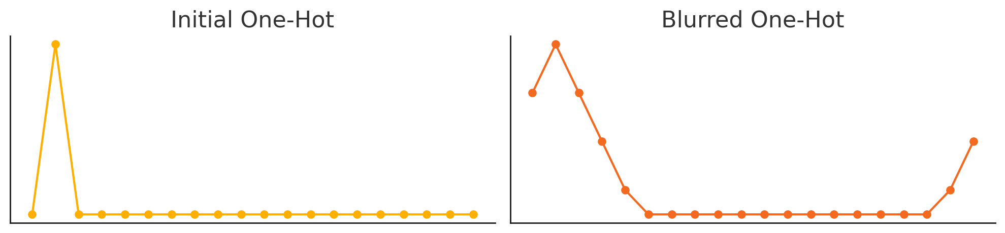
Wrapped, Blurry One-Hots
In training, the ‘target’ is a blurred one-hot of length 360,
- $\mathbf{v}$ is the original one-hot vector of length $n$
- $w$ is the phase width (an odd number)
- $i$ is the index of the non-zero element in the original one-hot vector
- $j$ is the current index in the blurred vector
The blurred vector $\mathbf{b}$ can be defined as:
$$ b_j = \max\left(0, 1 - \frac{2|j-i \bmod n|}{w}\right) $$
where $j \in {0, 1, …, n-1}$
E.g. for phase=1, the initial one-hot is
| 0 | 1 | 2 | 3 | 4 | 5 | … | 358 | 359 |
|---|---|---|---|---|---|---|---|---|
| 0 | 1 | 0 | 0 | 0 | 0 | … | 0 | 0 |
Once blurred with a phase_width of 7, it becomes
| 0 | 1 | 2 | 3 | 4 | 5 | … | 358 | 359 |
|---|---|---|---|---|---|---|---|---|
| 0.75 | 1 | 0.75 | 0.5 | 0.25 | 0 | … | 0.25 | 0.5 |
This reinforces the circular nature of the target space,
that 0 & 360 are not opposite but adjacent.
Training
The training for this model has taken a meandering path, and I’ve tried all sorts of tweaks and variations.
The basic setup for each run is:
-
Batch size of 1
- Each item is a full song, and each song is a different length
- Rather than trying to pad/stack/unpad, I decided to keep it simple and just train on one at a time
-
KLDivloss- Batchmean reduction
-
Adamoptimizer- Linear LR warmup of 5 epochs (20% -> full)
- Reduce LR by half after 5 epochs w/o improvement
Evaluation
Once the overall structure was established and I knew that it worked, I started running tests to determine the optimal parameters.
Phase Width
First, I ran 5 independent runs with various phase widths.
Parameters:
- Max 20 epochs
- Learning rate 1e-3 (with warmup)
| target width | 3 | 5 | 7 | 9 | 11 |
|---|---|---|---|---|---|
| best epoch | 17 | 11 | 13 | 17 | 10 |
| f-measure | 0.83 | 0.827 | 0.839 | 0.833 | 0.832 |
| cmlt | 0.8 | 0.796 | 0.807 | 0.804 | 0.798 |
| amlt | 0.872 | 0.862 | 0.874 | 0.871 | 0.86 |
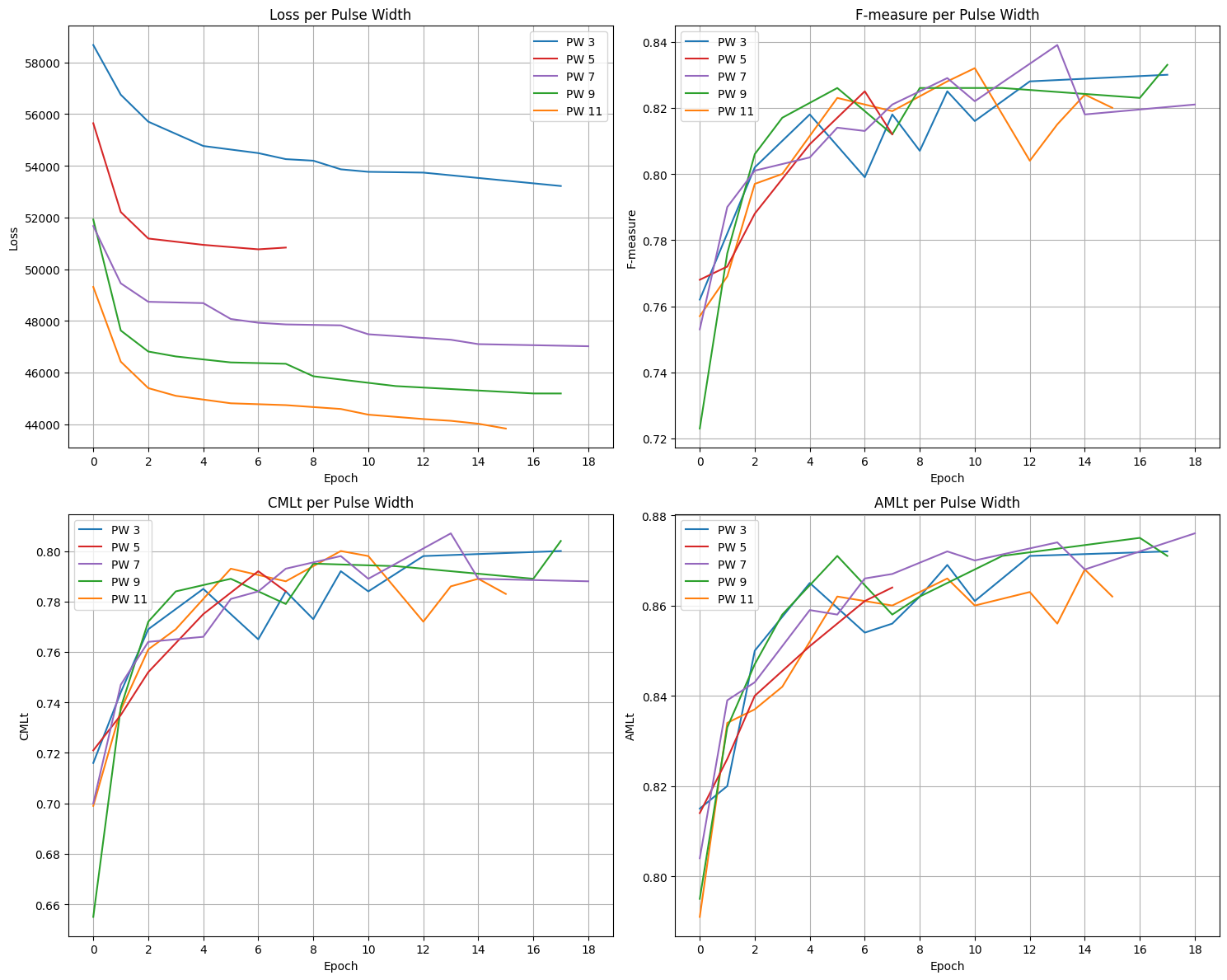
As shown, the pulse width had a clear effect on the magnitude of loss (bigger target = smaller loss), but it didn’t seem to have much of an effect on the predictive accuracy of the model.
Attention
Next, I tried removing attention.
Parameters:
- Epochs 0-19
- Learning rate 1e-3 (with warmup)
- Pulse width 7
- Epochs 20-39
- Learning rate 5e-4 (no warmup)
- Pulse width 7
| attention | no attention | |
|---|---|---|
| best epoch | 39 | 32 |
| f-measure | 0.848 | 0.855 |
| cmlt | 0.82 | 0.819 |
| amlt | 0.878 | 0.879 |
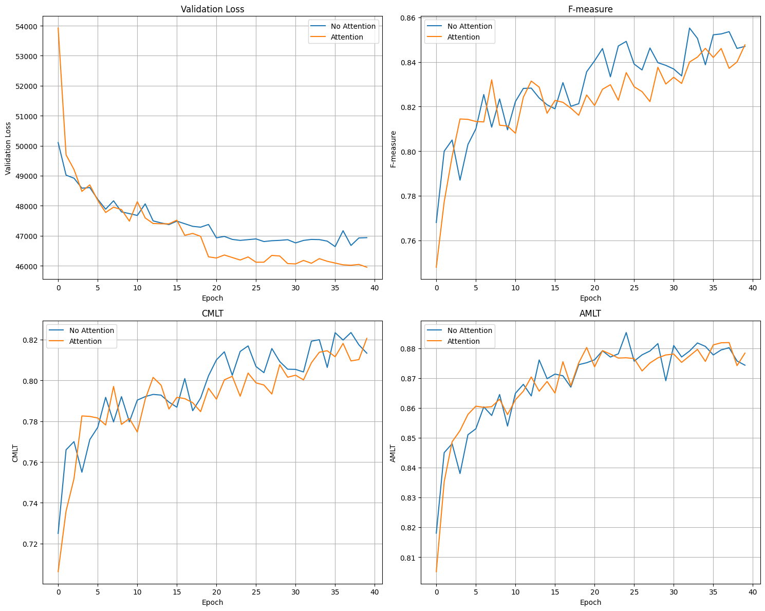
These results were surprising, as I thought attention would have a larger effect on the accuracy.
We can see that while the attention helped slightly with validation loss in the latter half of the test, it had little effect on the accuracy of the model (actually performing slightly worse overall).
My current theory on this is that the problem just isn’t hard enough to benefit from the added complexity, i.e. the audio data is not nuanced enough to contain ‘key words’, so the attention module learns to leave the TCN output mostly unchanged (don’t feel like testing this)
On one hand, I was a little disappointed because it seemed like a good idea, and initial tests seemed promising.
On the other, the attention module added quite a bit of heft, and in its absence, the model uses far less memory.
(Training w/ attention: ~20GB VRAM - 15it/s, training w/o attention: ~1GB VRAM, 25it/s)
Learning Rate
On both previous tests, I noticed that the accuracy metrics tended to jump around a lot.
My intuition was that the learning rate (1e-3) was too high, forcing it to take big steps that over/undershot the target.
So, I set up a few runs to test various rates (1e-5, 1e-4, 1e-3)
Note: the original paper used 1e-3
Parameters:
- 60 epochs
- Pulse width 7
| lr | 1e-5 | 5e-5 | 1e-4 | 5e-4 | 1e-3* |
|---|---|---|---|---|---|
| best epoch | 52 | 37 | 51 | 40 | 10 |
| f-measure | 0.807 | 0.853 | 0.849 | 0.854 | 0.837 |
| cmlt | 0.772 | 0.821 | 0.819 | 0.824 | 0.802 |
| amlt | 0.853 | 0.874 | 0.880 | 0.875 | 0.850 |
* In progress
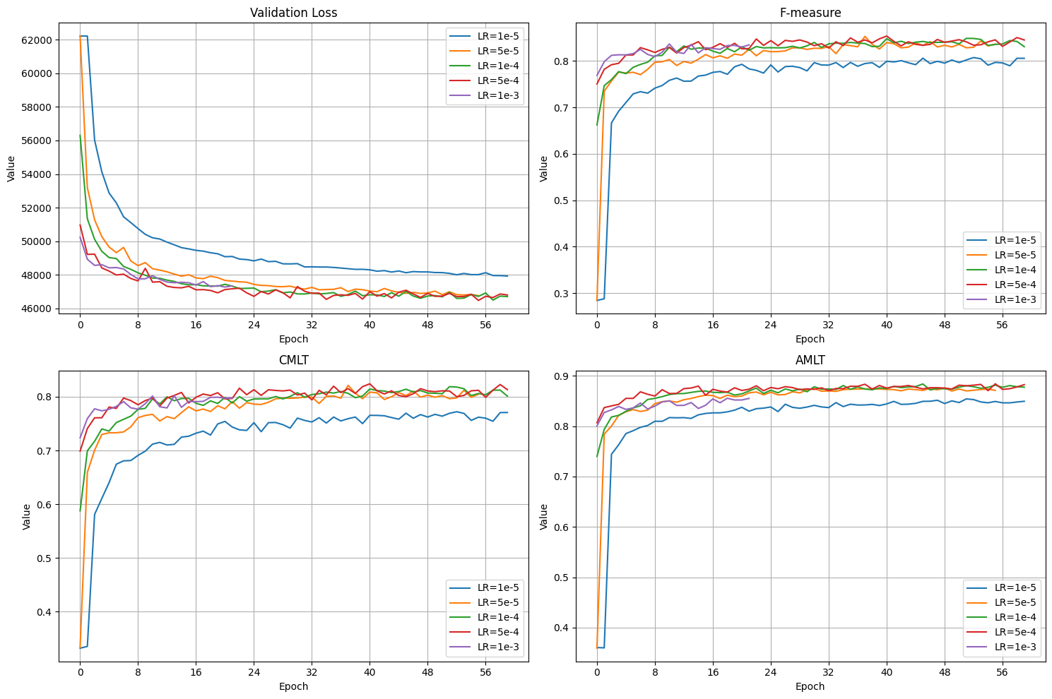
Evidently, the learning rate does not matter as much as I thought.
It looks like most runs converged pretty quickly on the same general trend (except for 1e-5 which seemingly hit a wall at about f=~0.8)
Interestingly, 1e-4 and 5e-4 appear to be tracing the exact same peaks and valleys in the loss chart from epoch 45-60
5e-4 looks like a good balance between stable and explorative, so I’ll be using that going forward.
Postproc
Should’ve done this one way sooner, but I tested putting the ‘phase targets’ through the HMM/cleaner and it scored 0.908.
This means that even if the model outputs the targets perfectly, its ‘accuracy ceiling’ is 0.908 (unless I fix the postproc)
So let’s try to fix the postproc.
First of all, there are a lot of ‘magic number’ parameters, especially in the cleaner functions. So we’ll do a grid search over various options for the parameters:
- HMM BPM confidence
- HMM distance threshold
- clean_beats interval threshold
- Interval mode threshold
- correct_beats ‘break points’
- Overlap
- Early
- Late
- Missed
- correct_beats nudge amount
Now, with 4 options per parameter, this grid has 262,144 combos, which is too many to check exhaustively.
So instead, I generated each combination of parameters, put them in a list, and shuffled it.
Now, I can watch the results as they come in, and get a decent estimate of the ‘shape’ of the data, honing in the param options as needed.
By sampling the random distribution across all variables, then plotting [var] vs f-measure for each parameter, I can approximate the effect of each variable.
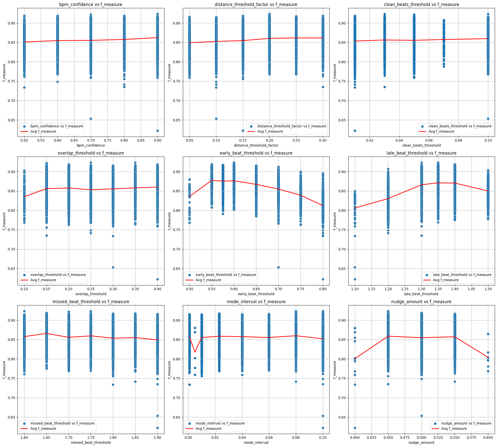
Thus, it becomes clear which variables have an effect on the overall accuracy (early/late beat threshold), and which do not (BPM confidence)
| params | original | optimized |
|---|---|---|
| f-measure | 0.854 | 0.881 |
| cmlt | 0.822 | 0.847 |
| amlt | 0.881 | 0.891 |