deeprhythm
github pypi
DeepRhythm is a convolutional neural network designed for rapid, precise tempo prediction for modern music. It runs on anything that supports Pytorch
(I’ve tested Ubuntu, MacOS, Windows).
Audio is batch-processed using a vectorized harmonic constant-q modulation (HCQM), drastically reducing computation time by avoiding the usual bottlenecks encountered in feature extraction.
Why?
I needed a way to accurately estimate tempo that was small & fast enough run on a Raspberry Pi.
I tried the estimators from librosa, essentia, and tempocnn, but all (open source) methods were unreliable and very slow.
So, I did some research and found this paper, describing a cnn that predicts tempo using an audio feature they call ‘Harmonic Constant-Q Modulation’.
In short, they perform a series of Constant-Q transforms over an 8s window, and rather than extracting the usual ‘pitch’ frequencies, they extract much lower ’tempo’ frequencies, e.g.
| freq range (Hz) | regular cqt | hcqm |
|---|---|---|
| max | 9397.27 | 4.76 (286bpm) |
| min | 32.70 | 0.5 (30bpm) |
When computed across eight frequency bands & six harmonics, it results in a 3d tensor that represents the relative strength of the tempos present in the audio.
This ’tempo cube’ can then be fed into a convolutional neural net that performs classification over 256 output classes (30-286bpm).
With this approach, the CNN barely has to do any legwork, and it functions more as a filter to reduce the dimensionality of the HCQM, i.e. instead of learning onset patterns, it just needs to interpret the relative strength of the bpm frequencies themselves.
Anyways, I couldn’t find any source code for the paper, nor any hcqm implementations, so I built my own. Here’s how it works.
HCQM
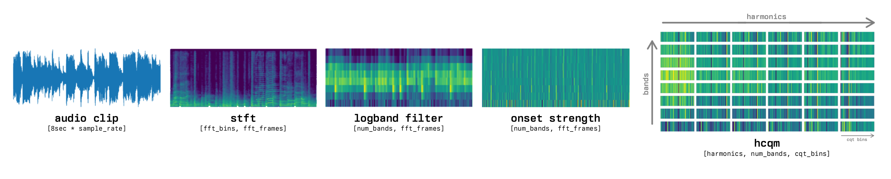
HCQM process for a single clip
Load a song
[duration*sample_rate]Chop and stack into 8s clips
[clips (duration//8), len_clip (8*sample_rate)]Compute STFT on slices
[clips, fft_bins (1+n_fft/2), fft_frames (len_clip/hop)]Compress into log-spaced bands
[clips, bands (8), fft_frames]Flatten into batch of band-signals
[clips*bands, fft_frames]Compute onset strength of band-signals
[clips*bands, fft_frames]Compute CQT (per harmonic)
[harmonics (6), clips*bands, cqt_bins (240), cqt_frames (1)]Reshape
[clips, cqt_bins, bands, harmonics]
Pre-process
Initially, I used librosa to compute the HCQMs (as mentioned in the paper), but I needed to compute 20-40 clips per song, for several thousand songs, which would’ve taken days.
So I rewrote the HCQM implementation with pytorch and nnAudio to run on the gpu instead.
The kernels / filters for each step are pre-computed and re-used, and with some careful flattening & reshaping it was possible to batch-process 50-100 songs at once, in less than a second (on a 4090).
Architecture
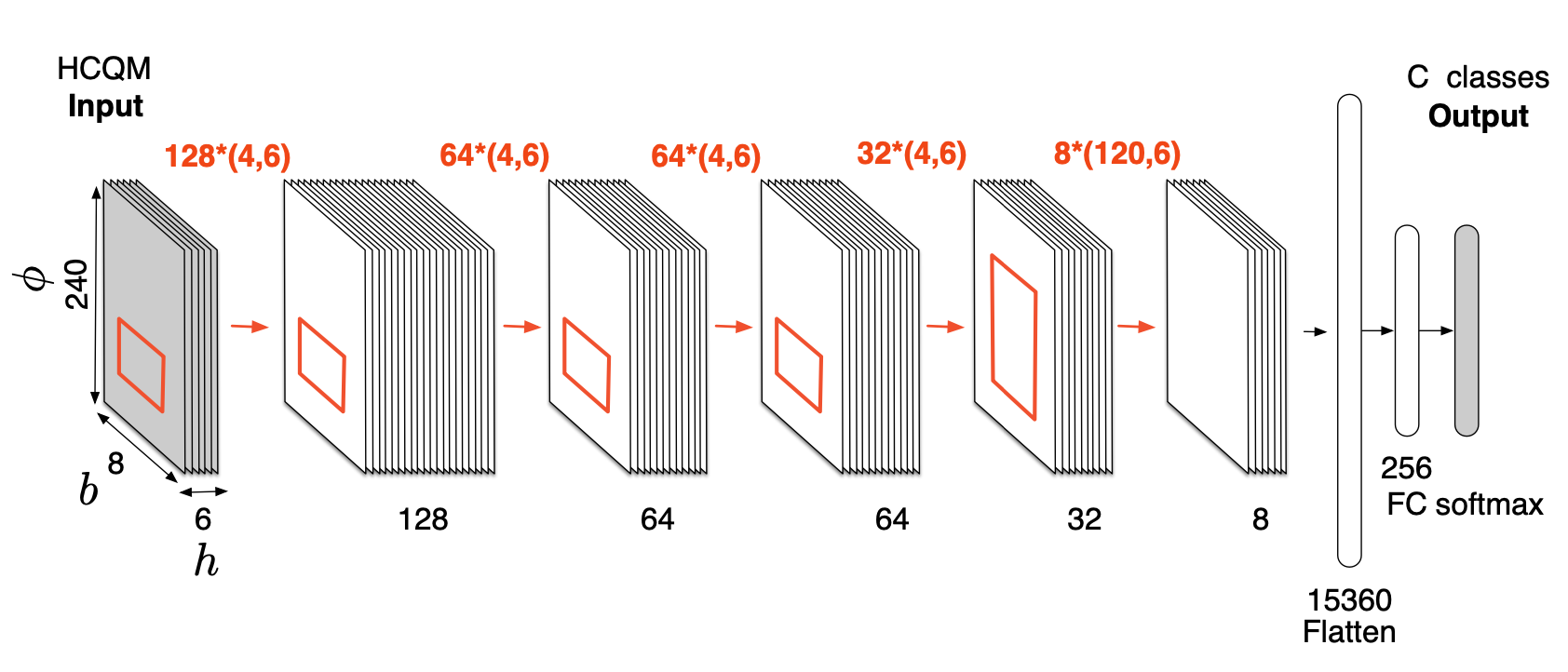
CNN architecture, from Foroughmand & Peeters
The architecture used is the same as the original paper, a pretty straightforward CNN.
- conv1
- input channels: 6
- output channels: 128
- kernel size: (4, 6)
- followed by batchnorm2d and relu activation
- conv2
- input channels: 128
- output channels: 64
- kernel size: (4, 6)
- followed by batchnorm2d and relu activation
- conv3
- input channels: 64
- output channels: 64
- kernel size: (4, 6)
- followed by batchnorm2d and relu activation
- conv4
- input channels: 64
- output channels: 32
- kernel size: (4, 6)
- followed by batchnorm2d and relu activation
- conv5
- input channels: 32
- output channels: 8
- kernel size: (120, 6)
- followed by batchnorm2d and relu activation
- fc1
- input features: 2904
- output features: 256
- followed by elu activation and dropout (0.5)
- fc2 (output layer)
- input features: 256
- output features: num_classes (default 256)
Data
For training data, I used giantsteps, ballroom, slakh2100, and a small subset of fma.
I ran the whole set through every other tempo predictor I could find, chose a ’true bpm’ by majority vote, then measured confidence as avg. distance between each predictor and the ‘winner’.
This allowed me to significantly clean up the dataset by removing multi-tempo / ambiguous / accoustic songs that cannot be predicted accurately
Training
The core setup was:
- batches of 256 (8 second clips)
CrossEntropyLossAdamoptimizer- learning rate 1e-5
- halves lr after 2 epochs no improvement
- quits after 5 epochs no improvement
Evaluation
| method | acc1 (%) | acc2 (%) | avg. time (s) | total time (s) |
|---|---|---|---|---|
| deeprhythm (cuda) | 95.91 | 96.54 | 0.021 | 20.11 |
| deeprhythm (cpu) | 95.91 | 96.54 | 0.12 | 115.02 |
| tempocnn (cnn) | 84.78 | 97.69 | 1.21 | 1150.43 |
| tempocnn (fcn) | 83.53 | 96.54 | 1.19 | 1131.51 |
| essentia (multifeature) | 87.93 | 97.48 | 2.72 | 2595.64 |
| essentia (percival) | 85.83 | 95.07 | 1.35 | 1289.62 |
| essentia (degara) | 86.46 | 97.17 | 1.38 | 1310.69 |
| librosa | 66.84 | 75.13 | 0.48 | 460.52 |
- test done on 953 songs, mostly electronic, hip hop, pop, and rock
- acc1 = Prediction within +/- 2% of actual bpm
- acc2 = Prediction within +/- 2% of actual bpm or a multiple (e.g. 120 ~= 60)
- timed from filepath in to bpm out (audio loading, feature extraction, model inference)
- I could only get tempocnn to run on cpu (it requires cuda 10)